





How to Evaluate the Long-Term Economics of an Asphalt Plant
Introduction
Many road construction contractors, asphalt producers, infrastructure companies, and investors tend to focus solely on comparing equipment quotes or rated production capacity when purchasing asphalt mixing plants, treating them simply as another piece of construction equipment. However, an asphalt mixing plant represents a significant long-term capital investment and must be evaluated from a long-term capital investment perspective, rather than as a mere equipment purchase. A single procurement decision often determines cash flow, production capacity limits, and project acquisition capabilities for the next five to ten years—or even longer.
The lowest equipment quote or the highest nameplate rated capacity does not necessarily translate to the best long-term economic benefits. The core factors determining the quality of a return on investment include: production demand, total initial investment, full life-cycle operating costs, actual equipment utilization rate, and project operating cycle. an asphalt mixing plant with a low quoted price but high fuel consumption and a high failure rate is likely to incur cumulative operating costs that exceed those of a more expensive yet energy-efficient and reliable unit within just a few years; conversely, an bitumen mixing plant with a massive rated capacity that remains idle for extended periods will cause fixed costs to erode unit profits. The true focus of an investment decision is not the equipment itself, but its ability to generate value for the enterprise throughout its entire service life.
This article will provide a practical investment evaluation framework for asphalt batching plants—including calculation formulas, case studies, and scenario analysis—rather than a standard equipment purchasing guide. We will explain total cost of ownership (TCO), production cost per metric ton of mix, break-even output, cash flow models, and scenario sensitivity analysis, using reproducible examples to demonstrate how to transform an “equipment quote” into a “conclusion on investment feasibility.” The ultimate conclusion is this: the most economically optimal investment solution is an asphalt mix plant configuration that aligns with your actual production needs and financial goals—not the unit with the most impressive specifications on paper.
Start with Realistic Production Demand, Not Rated Capacity
Key question: Can expected production demand support the investment?
The root cause of many procurement mistakes is substituting “how much capacity I hope to achieve” for “the output I can actually handle.” The first step in capacity planning is always an objective assessment of future production needs, not a preference for equipment specifications. The more realistic the demand assessment, the more meaningful the subsequent calculations of total investment, operating costs, and break-even points will be.
Estimate Annual Asphalt Production Demand
Annual production estimates cannot be set arbitrarily; they must be based on a comprehensive analysis of existing project contracts, market-aligned sales forecasts, and contracted project volumes. Cross-verification should prioritize the following three sources: First, contract orders that have already been signed and specify delivery dates and project volumes—this serves as the most reliable baseline for demand; second, potential projects currently being tracked that have a high probability of winning the bid, with demand calculated based on their likelihood of being awarded; third, the repurchase expectations and market expansion plans of existing customers, which serve as supplementary references. Setting production volumes based solely on “market intuition” or “industry peers’ production capacity” often leads to overestimating demand and underestimating risks.
At the same time, the seasonal nature of road construction must be fully considered: the number of effective construction days, daily production hours, and project delivery schedules all limit total annual output. Road construction is generally affected by temperature and the rainy season; in northern regions, work often halts for several months during winter, while the rainy season in the south also narrows the construction window. The effective daily production time is typically only 8 to 12 hours, not 24 hours. When calculating on an annual basis, these practical constraints must be factored in, rather than simply using “rated production capacity × 365 days.”
It is also important to distinguish between two types of output: one is asphalt mix for internal use in the company’s own road projects, and the other is commercial asphalt mix sold to external customers; the financial analysis logic for these two is entirely different. For in-house consumption asphalt mixing plants, profitability depends on the difference between “in-house production costs” and “the price of purchased asphalt mix,” as well as the value derived from controlling the construction schedule through in-house production capacity; for sales-oriented asphalt mixing plants, profitability depends on market prices, marginal contribution, and sales volume growth. The break-even points and sources of risk for these two types of operations are fundamentally different, so their classification must be clearly defined before conducting any calculations.
Distinguish Rated Capacity from Actual Production
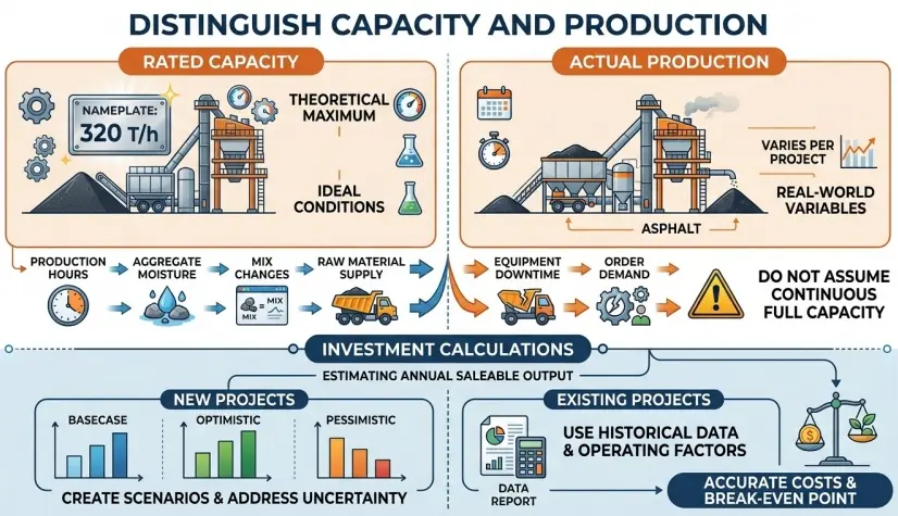
The rated capacity listed on equipment nameplates typically represents the theoretical production capacity measured under specific operating conditions; it does not reflect the actual output that can be sustained over the long term at a project site. Actual output is influenced by various factors, including production hours, aggregate moisture content, mix changes, raw material supply, equipment downtime, and order demand. Significant variations may exist between different projects, and there is no universal, fixed conversion ratio.
Therefore, in investment calculations, the annual saleable output should be estimated based on projected production shifts, effective production time, historical operating data, and project demand, rather than directly applying a fixed capacity utilization rate. For new projects lacking historical data, baseline, optimistic, and pessimistic scenarios can be established to reflect the uncertainty in actual output, and costs and the break-even point can then be calculated accordingly.
When conducting investment projections, never assume that the asphalt batch plant can operate at full rated capacity continuously throughout the year; otherwise, revenues will be severely overestimated.
Estimate the Expected Asphalt Mixing Plant Utilization Rate
Calculate actual annual output by combining available production hours with on-site operating conditions. The lower the utilization rate, the higher the fixed costs allocated per metric ton of mix. Here, utilization rate refers to the ratio of “actual productive time with output” to “theoretical available production time.” It integrates multiple factors—including demand saturation, construction seasons, breakdowns and maintenance, and production changeover losses—and serves as the core variable linking production capacity to actual output.
Investors need to assess the risks: If high-capacity equipment is purchased but future demand fails to fully utilize that capacity, idle capacity will continuously drive up unit costs, resulting in a waste of investment. For example, if large-scale equipment is purchased to meet peak-period production capacity but demand falls short during off-peak periods, the high depreciation and fixed expenses will continue to erode profits in years of low demand. When planning production capacity, one should weigh the “ability to meet peak demand” against the “cost burden during off-peak periods” to find an economically reasonable balance between the two.
Base capacity planning on realistic production demand, not theoretical maximum output alone.
Calculate the Total Initial Investment Before Comparing Asphalt Plant Economics
Key question: What is the full investment required to get the asphalt mixing plant operational?
To compare the cost-effectiveness of two proposals, it is essential to ensure that the “basis for calculation” is consistent. Many comparisons are skewed because they only consider the base price of the equipment, while overlooking the full range of costs required to “get the equipment up and running”—including ancillary systems, site preparation, transportation, commissioning, and working capital. Total Initial Investment = Equipment Purchase and Ancillary Systems + Site Preparation, Installation, and Commissioning + Transportation, Customs Clearance, and Pre-Operational Preparation + Working Capital and Financing Arrangements. Each item must be listed separately and calculated individually.
Equipment Purchase Price and Required Configuration
Quotes should not only include the main unit but also cover the entire set of auxiliary systems required for the project. Distinguish between essential standard configurations and optional configurations that can be added later. The total investment for an asphalt mixer plant typically includes aggregate batching and conveying, drying drums, combustion systems, mixing towers, powder and asphalt supply systems, dust collection and environmental protection systems, and electrical control and metering systems; Differences in fuel selection (heavy fuel oil/natural gas/burners) and environmental protection standards will significantly affect the quoted price.
Before comparing quotes from multiple suppliers, standardize the scope of equipment across all proposals to avoid misjudgments caused by direct comparisons of “bare equipment” prices—such as when Quote A excludes powder silos and dust collection systems, while Quote B includes a full set of supporting equipment. The correct approach is to create a standardized “Equipment Configuration List” and require each supplier to quote based on this same list, then compare the quotes accordingly. For modules that are truly optional or can be deferred, they should be clearly marked separately and defined consistently, rather than vaguely included in the total price.
Site Preparation, Installation, and Commissioning
Site grading, equipment foundations, utility connections, equipment installation, and no-load and load testing all require capital investment. A batch asphalt mixing plant typically requires a paved area of a certain size for storing aggregates and finished products, as well as for positioning the mixing unit and auxiliary equipment. Site grading, foundation pouring, drainage systems, access roads, electrical capacity upgrades, and water supply connections are all mandatory expenses that must be completed before production begins.
Additionally, project-specific engineering design and plant infrastructure construction involve many cost items that are not listed on equipment quotations and are easily overlooked. For example, master planning and process design, environmental protection facilities and acceptance inspections, fire safety and security facilities, as well as office and living facilities—each of these represents a significant expense on its own, and when combined, they may account for a substantial portion of the total investment. When developing an investment model, these “hidden ancillary costs” should be made explicit, estimated item by item, and incorporated into the total investment.
Transportation, Import Duties, and Start-Up Expenses
Cross-border procurement involves domestic and international logistics, customs clearance, and import duties. Costs such as ocean and land freight, port loading and unloading, customs brokerage, import duties and value-added tax (VAT), and cargo insurance are unavoidable expenses for imported equipment. Factors such as inland transport distance, whether the cargo exceeds standard dimensions, and the need for special transportation solutions can all significantly increase logistics expenses. For locally procured equipment, freight costs from the supplier to the plant site and hoisting fees must also be considered.
Pre-production costs also include the initial spare parts package and operator training. All estimates must be based on the actual conditions at the project site; generic estimates should not be used. The initial start-up often requires stockpiling of wear-and-tear parts and critical spare parts to avoid downtime while waiting for parts. Before a new plant goes into operation, training for operators and maintenance personnel, as well as materials and consumables used for commissioning during the trial production period, should also be included. Tax rates, logistics rates, and labor rates vary significantly across different countries and regions; therefore, actual local quotes should be used whenever possible rather than general empirical values.
Working Capital and Financing Requirements
The procurement of raw materials, inventory, and accounts receivable all require working capital. As soon as a batch mix asphalt plant begins operations, it requires ongoing funds for the procurement of aggregates, asphalt, fuel, and auxiliary materials. At the same time, sales often involve credit terms, resulting in a cash tie-up where payments are advanced before receipts are collected. Working capital requirement = average inventory tie-up + accounts receivable tie-up – accounts payable credit limit. Given the significant scale of this requirement, it must be included in the initial capital planning.
Consider the cash flow pressure resulting from supplier payment terms and customer collection cycles. When comparing multiple options, funding costs—such as interest on financing—must be accounted for using a consistent methodology within the financial model. Whether funding comes from self-raised capital, bank loans, or finance leases, there is a cost associated with using these funds; when comparing different investment options, a consistent financing structure and discounting methodology should be applied to avoid distorted comparisons caused by differing treatments of funding costs.
For more information on the relationship between procurement quotes, configuration scope, and the complete investment budget, please refer to the Your Complete Asphalt Mixing Plant Buying Guide.
Key Point: Compare complete project investment requirements rather than equipment prices alone
Understand the Operating Costs That Shape Long-Term Economics
Key Question: Which recurring expenses have the greatest effect on long-term financial performance?
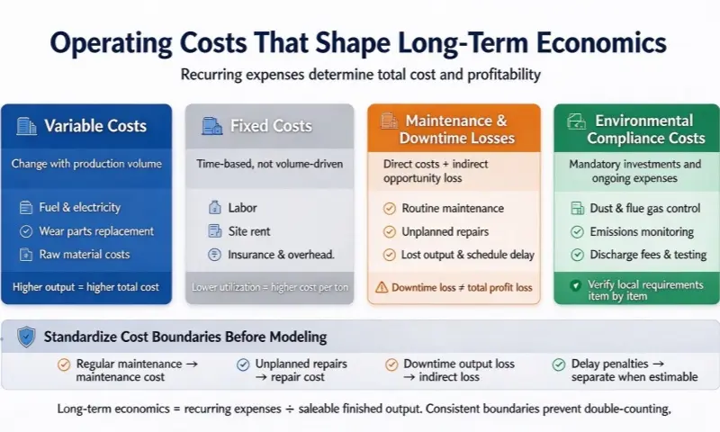
Procurement is a one-time expense, while operations involve ongoing costs throughout the equipment’s lifespan. Long-term economic viability is primarily determined by the structure of operating costs. Operating costs can be broken down into four categories: “variable costs that fluctuate with output,” “fixed costs incurred over time and based on scale,” “maintenance and downtime losses,” and “environmental compliance costs.” These should be accounted for separately and evaluated individually for their impact on profitability.
Variable Operating Costs per Ton
Variable costs fluctuate in tandem with asphalt mix output: energy costs such as fuel consumption (based on local fuel prices) and electricity; replacement costs for wear-and-tear parts; and raw material costs included according to the cost model’s scope. The higher the output, the higher the total expenditure in this category, but the unit variable cost remains relatively stable. Fuel and electricity costs typically account for the largest portion of a batch mix plant’s operating costs and directly determine the energy cost per metric ton of mix; therefore, the plant’s combustion efficiency, drying process, and levels of heat retention and waste heat recovery have a significant impact on long-term economic efficiency.
Wear-prone and wear-resistant parts (such as mixing blades, liners, screens, and conveyor belts) are consumed in tandem with production volume; their unit prices and service lives vary depending on equipment quality, making them key indicators for assessing whether “cheap equipment is truly cost-effective.” Whether raw material costs are included depends on the scope of your cost model: if calculating “on-site production costs,” aggregates and asphalt may be excluded; if calculating “full cost of the mix,” they must be included. Different scopes yield different conclusions; consistency must be maintained when making comparisons.
Fixed Costs and Time-Based Operating Expenses
Regardless of output levels, these costs occur on a regular basis: labor for production shifts, site rent, insurance, allocated management expenses, and expenditures for periodic maintenance and repairs carried out on a fixed schedule. Even if output falls short of expectations, fixed costs continue to accrue. Labor, rent, insurance, and management salaries are incurred monthly and are independent of output; Once determined, these costs constitute a rigid burden on operations.
The key implication of fixed costs for long-term economic viability is that they must be allocated across the “output of saleable finished goods.” When demand declines or capacity utilization is low, fixed costs do not disappear; instead, they cause the allocated cost per metric ton to rise sharply, directly eroding profit margins. Therefore, when assessing long-term economic viability, both the absolute amount of fixed costs and their impact as capacity utilization fluctuates must be factored in.
Maintenance, Repairs, and Losses from Unplanned Downtime
Routine maintenance, replacement of parts, and repairs for sudden breakdowns constitute direct maintenance costs. Proper preventive maintenance can reduce the probability of sudden breakdowns, but it itself requires investment in labor, spare parts, and downtime; these expenses should be included in the model as predictable periodic costs rather than treated as contingencies.
The losses resulting from downtime can be divided into two categories: first, the cost of repair materials and labor; second, indirect economic losses caused by reduced output and project schedule delays—the latter of which is often more easily overlooked. The direct loss from a single day of downtime is the repair cost, while the indirect losses include the profit that would have been generated that day, the risk of breach of contract due to project delays, and the erosion of customer trust. For projects with strict deadlines, the hidden value of highly reliable, low-failure-rate equipment far exceeds the difference in repair costs on paper. When evaluating options, one should consider both “the reliability of the equipment itself” and “the impact of downtime on business operations,” rather than simply comparing repair quotes.
Environmental Compliance and Site-Specific Costs
Dust collection systems, emissions monitoring equipment, and local environmental and emissions regulations are all mandatory investments. Environmental policies vary significantly across regions; before project modeling, it is essential to confirm the regulatory requirements at the project site and incorporate compliance costs into the calculations. Many countries and regions have strict standards for dust, flue gas, and noise emissions from asphalt plants; failure to meet environmental standards not only results in fines but may also lead to orders to suspend operations for corrective action.
Environmental compliance costs include one-time investments (such as dust collection bags, activated carbon adsorption systems, enclosed silos, and noise reduction facilities) as well as ongoing operating expenses (monitoring, consumables, discharge fees, and third-party testing). Requirements vary significantly by region; for example, limit values for particulate matter, SO₂, and NOx differ, as do regulations regarding whether online monitoring is required and whether nighttime production is restricted. All of these factors should be verified item by item based on the actual regulations in the project’s location, rather than applying general practices from the region where the headquarters is located.
Standardize Cost Categories and Accounting Boundaries
Before establishing a cost model, cost categories and accounting boundaries should be standardized to prevent the same expense from being double-counted.
| Cost Item | Recommended Approach |
| Regular maintenance and scheduled replacements | Include in maintenance and repair costs according to established accounting criteria |
| Repairs for Sudden Failures | Include in repair costs to avoid duplication with the maintenance budget |
| Production Losses Due to Downtime | Assess separately as an indirect economic impact |
| Penalties for Delays, etc. | Include separately when they are likely to occur and can be reasonably estimated |
The reduction in production volume caused by downtime is not equivalent to the total loss of profit. If production can be made up after the downtime or if market demand is insufficient, the actual economic loss will be lower than the profit corresponding to the theoretical output. The term “profits that would have been generated,” as mentioned in the text, should be understood as an opportunity cost calculated based on make-up production capacity, order demand, and actual marginal contribution; losses should not be estimated directly using the output value corresponding to rated production capacity.
If evaluating the economic viability of the asphalt batch mix plant equipment itself, equipment-related costs may be accounted for separately; if evaluating the profitability of the entire asphalt mixture production operation, corresponding raw material costs and other production expenses should be included.
Key Point: The long-term economic viability of an asphalt mixing plant’s operation is determined by both ongoing expenses and the amount of marketable finished product these costs can generate; standardize cost metrics before modeling to avoid double-counting.
Evaluate the Total Cost of Ownership (TCO) Over a Defined Period
Key question: How much will the investment cost over its expected evaluation period?
Long-term economic viability cannot be determined by looking solely at equipment quotes, nor can it be determined by examining the costs of a single year. Total Cost of Ownership (TCO) places investment, operation, maintenance, and disposal within a single timeframe for unified calculation; it is the foundational tool for determining “which solution is more cost-effective overall.” It answers not “how much will it cost to buy this unit,” but rather “how much will it cost in total to own and operate this equipment over the evaluation period.”
Choose a Consistent Evaluation Period
Determine the evaluation period based on the company’s investment plans and the expected useful life of the equipment, rather than relying on some “industry standard.” For example, you can establish separate 5-year and 10-year projection scenarios to observe how costs, cash flows, and residual values over different time horizons affect investment decisions. If the period is too short, it will exaggerate initial investments and underestimate the long-term maintenance and operational advantages; if the period is too long, it will be heavily influenced by technological and market changes, reducing the reliability of forecasts.
When comparing different bitumen batch mix plant solutions, the evaluation period must remain consistent; otherwise, the calculation results will not be comparable. If one set of equipment has a 10-year lifespan while another may require major repairs or replacement after 8 years, “future reinvestments” must be factored into a unified timeframe, rather than simply comparing their respective nominal lifespans.
Build a Lifecycle Cost Model
Life-Cycle Cost Formula:
Life-Cycle Cost = Initial Investment + Operating Costs + Maintenance Costs + Other Related Costs – Residual Value at the End of the Period
Distinctions in Calculation Principles:
- Total Cost of Ownership (TCO) over the Entire Evaluation Period: Includes all initial capital investments, operating, and maintenance costs within the period, minus the residual value at the end of the period.
- Annual Cost / Cost per Metric Ton: Capital costs must be allocated to the corresponding periods using a uniform methodology and then matched with operating costs and saleable output for the same period.
- Cash Flow and NPV Analysis: Investment expenditures, operating cash flows, and residual value at the end of the period are recognized based on the actual timing of cash outflows; financing costs and the discount rate must follow consistent financial conventions, and double-counting is prohibited.
Important Note: Depreciation is solely a method of cost allocation for accounting purposes and does not constitute an actual cash outflow. The calculation logic for per-metric-ton costs under accounting standards differs from that for project cash flow calculations; therefore, the same methodology cannot be directly applied to both. This prevents the duplicate calculation of initial investment, depreciation, and financing costs, as well as the mixing of data from different time periods.
Summarize all expenses, including capital investment, operations, and maintenance; Estimate the residual value of the equipment at the end of the evaluation period; standardize the statistical criteria for financing, taxes, and working capital to avoid double-counting. Residual value should be estimated based on the actual resale or continued-use value of the equipment at the end of the evaluation period, rather than as a fixed percentage of the original investment; either financing interest or the opportunity cost of equity capital must be used, and the criteria for taxes (including import duties, value-added tax, and income tax impacts) must be consistent throughout to prevent the same expenditure from being counted twice.
It is important to distinguish that TCO is a cost metric reflecting “total expenditure” and is not equivalent to return on investment; whereas NPV (Net Present Value) is a discounted net cash flow metric that typically incorporates both investment expenditures and operating cash inflows, reflecting “value creation after accounting for the time value of money.” The two serve different purposes and should not be confused. Financing interest, taxes, working capital, and residual value at the end of the assessment period should all be treated according to consistent financial criteria.
Compare Alternatives on the Same Basis
All alternative options should use the same annual production target, mix specifications, and evaluation period. Standardize the scope of cost calculations and comprehensively compare full life-cycle costs, production capacity, and on-site O&M requirements; do not focus on a single metric alone. If Option A has a lower total cost but insufficient capacity, requiring additional outsourcing, while Option B has a higher total cost but ample capacity, the “outsourcing gap cost” must be factored into Option A before making a comparison.
Evaluation metrics must be used in combination: total life-cycle cost reflects “overall expenditure,” cost per metric ton reflects “unit economics,” and production capacity and reliability reflect “ability to fulfill commitments on time.” These three factors collectively determine a solution’s suitability. Drawing conclusions based solely on a single favorable metric can lead to a narrow, one-sided view.
Account for the Time Value of Money
Introduce the concepts of discounted cash flow and net present value (NPV). Costs and revenues occurring in different years do not have the same financial value. Calculations must be performed using a discount rate that matches the company’s required rate of return on investment. One yuan today is worth more than one yuan next year because funds available today can generate returns; only by discounting cash outflows and inflows from future years to their present value using the discount rate can a fair comparison be made between investment alternatives with different time distributions.
The discount rate is typically set at the company’s weighted average cost of capital (WACC) or a predetermined minimum required rate of return (e.g., 8%–12%). Discounting is particularly important when comparing proposals characterized by “high initial investment and high returns in later years”: without discounting, proposals with higher future returns and lower initial investment would be significantly overestimated. It is recommended to calculate both NPV and internal rate of return (IRR) in addition to TCO to validate the feasibility of the investment from different perspectives.
For further insight into the economic differences between building your own asphalt mixing plant and other supply methods, please refer to “Why You Should Buy Your Own Asphalt Plant.”
Key Points: TCO provides a comprehensive picture of total long-term expenditures; discounted cash flow (DCF) assesses the true value of costs and revenues occurring at different points in time.
Calculate Cost per Ton and Break-Even Production Volume
Key question: How much production is needed to make the investment economically viable?
Total life-cycle cost answers the question “How much will it cost in total?”, while cost per metric ton and break-even production volume answer “How much output does this investment require to become self-sustaining?” Only by combining these two can capital investment be aligned with an operationally feasible and verifiable production volume threshold. Unit cost reveals economic viability, while the break-even point defines the safety margin.
Calculate the Asphalt Plant-Related Cost per Ton
Formula:
Cost per metric ton = Total costs included in the calculation ÷ Total metric tons of saleable finished mix
The scope of the calculation must be clearly defined: whether it includes only mix plant-related costs or encompasses the full production costs of the asphalt mixture. When comparing different batching plant solutions, the scope of cost calculations must be completely consistent. If comparing “on-site costs,” both calculations should include only on-site depreciation, energy, labor, and maintenance; if comparing “full costs of the mixture,” both should include raw materials such as aggregates and asphalt. If the scopes are mixed, the comparison results become meaningless.
The numerator, “total cost,” consists of the allocated capital costs plus operating costs for the corresponding evaluation period; the initial investment is allocated over the period according to the selected amortization method, rather than being directly included in full in a single period’s costs.
It is also important to distinguish between “actual output” and “marketable output”: actual output refers to the asphalt mixture actually produced; “Saleable output” refers to finished material that meets the project’s quality requirements and is ready for delivery or use; the two are not necessarily equal. The denominator “metric tons” must be the actual saleable output for the same period, not the rated production capacity or total actual output. Unit costs should use the output metric that matches the cost model; using rated production capacity as the denominator significantly underestimates the true unit cost, which is a common misconception.
Calculate the Break-Even Production Volume
For the external sales of asphalt mixtures, the break-even production volume can be estimated using the following formula:
Break-Even Production Volume = Total Fixed Costs ÷ Margin per Metric Ton
Where: Margin per Metric Ton = Selling Price per Metric Ton – Variable Cost per Metric Ton
This formula applies to a simplified sales business model and requires two prerequisites: first, fixed costs and marginal contribution per metric ton must be based on the same evaluation period and statistical criteria; second, the marginal contribution per metric ton must be positive, and the selling price and unit variable cost must be reasonably estimable within the relevant production volume range. The calculation result represents the sales volume required to cover the relevant fixed costs under given assumptions; it should not be directly interpreted as the production volume at which the entire initial investment has been recovered.
For road construction contractors that produce materials for their own use, the following comparison criteria must be clearly defined prior to calculation: first, the complete, relevant costs of producing asphalt in-house; second, the delivered cost of directly purchasing finished asphalt from external suppliers; and third, the quantifiable impacts of the in-house production option, such as transportation costs, waiting time, or supply reliability. In-house production is economically viable only when the full cost of in-house production is lower than the delivered cost of externally purchased finished asphalt, and when the contractor’s own production capacity can ensure project completion within the scheduled timeframe—this helps avoid the misconception that “lower equipment operating costs” necessarily mean “the in-house production option is always more economical.”
Understand the Impact of Low Plant Utilization
A decline in output leads to an increase in fixed costs allocated per metric ton. Idle capacity, project delays, and short construction seasons can all result in insufficient utilization. Investors must verify whether projected market demand is sufficient to support the minimum output required for the investment. Utilization is one of the most sensitive variables in break-even analysis: when fixed costs remain constant, a 10% drop in output causes unit costs to rise significantly, thereby narrowing profit margins.
In practice, the “break-even production volume” should be compared with the “realistically achievable production volume”: if the realistically achievable production volume remains below the break-even point over the long term, it indicates that the investment scale is too large, and capacity should be reduced or the business structure adjusted; if the achievable production volume is only slightly above the break-even point, it indicates an insufficient profit buffer and weak risk resilience. This comparison directly reflects the feasibility and vulnerability of the investment.
Illustrative Example: How Annual Production Affects Cost per Ton
The table below is a hypothetical example; actual figures depend on the project and local operating conditions:
| Annual Production Volume | Annual Fixed Costs | Allocated Fixed Costs per Metric Ton |
| 40,000 metric tons | $200,000 | $5.00/metric ton |
| 60,000 metric tons | $200,000 | $3.33/metric ton |
| 80,000 metric tons | $200,000 | $2.50/metric ton
|
The table shows only the allocation of fixed costs and does not include variable costs. As production volume increases, fixed costs are spread over a larger volume, causing unit fixed costs to decrease continuously. Take annual fixed costs of $200,000 as an example: at an annual output of 40,000 metric tons, the cost per metric ton is $5; when output doubles to 80,000 metric tons, the cost per metric ton drops to $2.50—simply by increasing capacity utilization, the unit cost can be cut in half. This also illustrates the reverse: when capacity utilization is insufficient, the same fixed costs cause unit costs to rise rapidly, directly undermining price competitiveness.
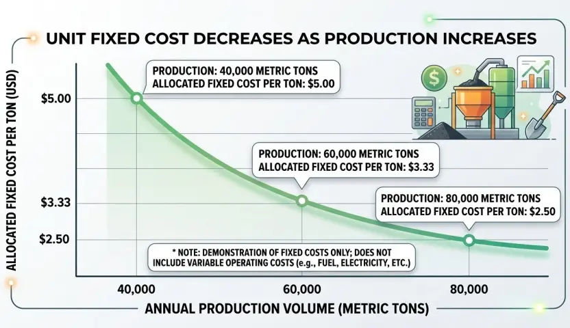
It is important to note that this table illustrates only fixed cost items; in actual operations, unit full costs must also include variable costs per metric ton (such as fuel, electricity, wear-and-tear parts, raw materials, etc.). When assessing overall economic viability, fixed and variable costs should be combined and compared against market-acceptable prices.
Key Point: Break-even analysis links capital investment to actual production demand and quantifies the investment risk resulting from insufficient capacity utilization.
Test Investment Returns Under Different Scenarios
Key question: Will the investment remain viable if actual conditions differ from expectations?
Any investment projection is based on assumptions, yet reality rarely unfolds exactly as assumed. The purpose of scenario analysis is not to answer “what is most likely to happen,” but rather to determine “whether the investment remains viable even if conditions worsen.” By constructing multiple scenarios, identifying sensitive variables, and calculating payback periods and critical conditions, investors can see the true boundaries of downside risks beyond optimistic projections.
Build Base-Case, Upside, and Downside Scenarios
- Base-Case Scenario: Production volume, costs, and project duration are based on the most reasonable and likely forecasts. The base-case scenario should be a “neutral and prudent” projection—neither overly optimistic nor deliberately pessimistic—serving as a baseline for comparison.
- Optimistic Scenario: Market demand is higher, equipment utilization exceeds expectations, and selling prices or cash collections are more favorable. This scenario is used to assess the potential upside and help determine whether the investment possesses sufficient upside flexibility.
- Pessimistic Scenario: Output declines, operating costs rise, equipment commissioning is delayed, and cash collections are delayed. This scenario is used for stress testing to determine whether the investment remains viable under the most adverse reasonable conditions and to quantify the magnitude of potential losses.
The values of key variables across the three scenarios must form a coherent system and be mutually consistent (for example, in the pessimistic scenario, the assumptions of low output, high costs, and extended construction periods should all hold simultaneously); they should not be pieced together by selecting extremes to create a “worst-case stack,” as this would distort the calculations.
Test the Variables That Matter Most
Conduct sensitivity analysis on the following key variables: annual production volume and equipment utilization rate; fuel and energy prices; maintenance expenses and unplanned downtime; project delays and customer payment cycles; financing costs; and working capital pressure. Observe the extent to which investment return metrics fluctuate with changes in these variables to identify risk points.
A common approach to sensitivity analysis is “single-variable perturbation”: based on the baseline scenario, vary only one key variable at a time (e.g., production volume ±20%, fuel prices ±15%) and observe the extent of changes in NPV, internal rate of return, or payback period. The variable with the greatest impact on the results represents the risk point that requires the most attention in the investment and is most worthy of effort to verify and manage. Typically, fuel prices and utilization rates are the two variables most sensitive to the economic performance of an asphalt plant and should be tested first.
Estimate Payback Period and Cash Flow
When annual net cash inflows are relatively stable, a simplified formula can be used to estimate the static payback period:
Static Payback Period ≈ Initial Investment ÷ Annual Net Cash Inflow
If there are significant variations in the project’s annual cash flows (such as large fluctuations in output, profits, accounts receivable, or maintenance expenses), simply dividing the initial investment by the net cash flow of a single year can lead to misleading conclusions. Instead, net cash flows should be accumulated year by year to determine when the cumulative cash flow covers the initial investment. For long-term investments, discounted cash flow (DCF) and net present value (NPV) can also be used to assess the time value of money. It is important to emphasize that the payback period, NPV, and return on investment (ROI) reflect different aspects and should not be used interchangeably.
Additionally, to evaluate ROI, the following formula can be used:
ROI = Net Investment Return ÷ Investment Cost × 100%
When calculating ROI, it is essential to clearly define the scope of returns—whether they represent annual returns or cumulative returns over the entire evaluation period—and to specify the scope of investment costs, including whether they encompass ancillary facilities, pre-production preparations, and other related expenses. Investment decisions regarding multi-year asphalt mixing plants should not rely solely on the ROI metric; instead, a comprehensive assessment should be made by combining cash flow analysis, net present value (NPV), and the payback period.
Net Present Value (NPV) Formula:

Where is the net cash flow in period t, r is the discount rate, and n is the number of evaluation periods; cash flow in period 0 generally includes initial investment expenditures.
Identify the Conditions That Could Change the Investment Decision
Determine the point at which demand must fall for the project to shift from profitable to unfeasible; assess whether the company can withstand the impact of rising costs and delayed cash collections. Identify which assumptions require further verification before capital is committed. Critical condition analysis typically yields a set of “thresholds”—such as the minimum break-even production volume, the upper limit for oil prices, and the tolerable decline in unit price—which together constitute the investment’s “safety margin.”
If a key assumption—such as future demand or fuel price trends—is difficult to verify, and this assumption directly determines the investment decision, it should be listed as a “priority verification item.” Before signing a contract or committing funds, reduce uncertainty by conducting additional market research, securing more certain orders, or taking measures such as locking in fuel procurement or adjusting payment terms. The value of an investment decision lies in transforming “uncertainty” into “manageability.”
Equipment upgrades are one possible path to improving the performance of existing investments, but they may not be suitable for all projects. For reference, see “Tips for Upgrading an Asphalt Plant for Better ROI.”
Key Point: Reliable investment decisions must be justifiable under both expected and adverse scenarios and cannot rely solely on optimistic forecasts.
How Asphalt Plant Configuration Can Influence Long-Term Economics
Key question: Which equipment configuration best fits the project’s financial and operational requirements?
Applying the same economic evaluation framework to different configurations will yield different conclusions. Production capacity, whether the plant is fixed or mobile, and whether it includes a RAP recycling module will all simultaneously affect the initial investment, operating costs, and suitable application scenarios. Configuration selection should be based on project-specific economic calculations, rather than generalizations such as “bigger is better” or “a certain type is guaranteed to save money.” Evaluations should focus on how different configurations alter cash flow, cost structures, and investment risks, rather than merely listing equipment specifications.
| Configuration Factors | Key Points for Economic Assessment |
| Production Capacity | Can the additional output cover the increased investment and operating costs? |
| Mobility | Can the costs of relocation, transportation, and assembly/disassembly be offset by project revenues? |
| RAP Recycling Module | RAP procurement costs, material savings, additional energy consumption, equipment investment, and regulatory requirements |
| Automation and Control Systems | Quantifiable labor savings, production stability, and changes in downtime or quality losses |
Aligning Production Capacity with Actual Demand
Balance equipment investment with actual production needs, and quantify the economic losses resulting from idle capacity. Dispelling a common misconception: A asphalt hot mix plant with higher capacity does not necessarily result in lower costs per metric ton. If demand is insufficient, high-capacity equipment can actually drive up unit costs. This is because higher capacity often corresponds to higher initial investment, larger site requirements, and a higher baseline for energy consumption; once demand cannot be fully met, the disadvantages of fixed-cost allocation become apparent.
The correct approach is to “base production on demand”: First, determine the realistic annual production range, then select a model capable of covering that range with high utilization rates. If future demand is likely to grow, prioritize models with “scalable configurations and expandable modules” to secure room for future upgrades with a lower initial investment, rather than deploying high-capacity equipment from the start.
Evaluate Mobility Against Project Duration and Relocation Needs
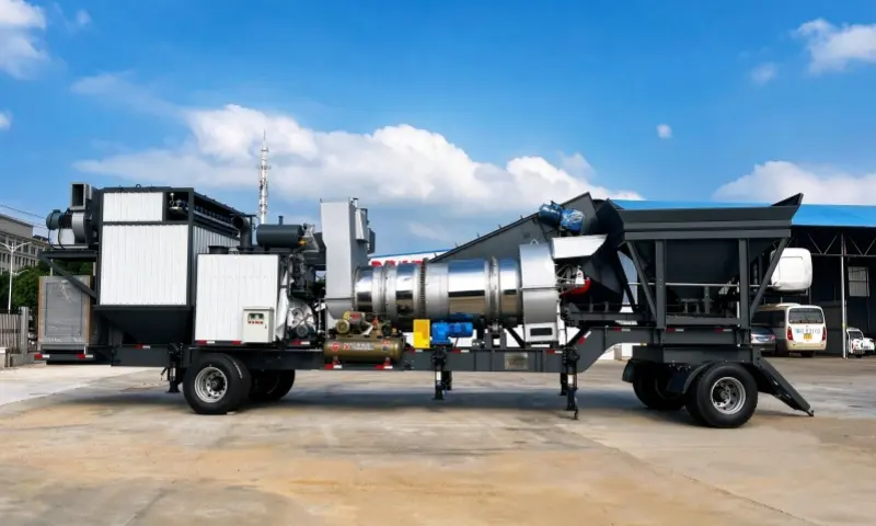
If projects are dispersed and require multiple relocations, evaluate the total costs of disassembly, transportation, and reinstallation. The advantage of mobile/relocatable batching plants lies in their ability to rotate between multiple job sites, transforming “building a single plant” into “reuse across multiple projects” and reducing the repetitive investment of building a separate plant for each project; however, each relocation incurs costs for disassembly, transportation, and reinstallation and commissioning, and frequent relocations may affect equipment stability and overall service life.
For long-term production at a fixed location, the focus should be on evaluating the long-term economic efficiency of a stationary asphalt mixing plant. Stationary plants eliminate the costs of repeated relocations and allow for the construction of more comprehensive site and environmental protection facilities, making them suitable for scenarios requiring long-term, stable supply or for the company’s own long-term projects.
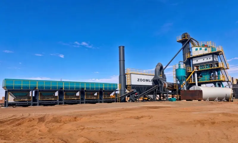
For projects with short construction periods, dispersed locations, and the need for multiple relocations, mobile asphalt plant or relocatable asphalt mixing plants may offer greater economic advantages, as the equipment can be reused across multiple projects. For long-term, centralized production scenarios with stable demand, stationary asphalt mixing plants may offer better long-term economic efficiency by reducing the costs associated with repeated relocations. Ultimately, a decision should be made only after comparing equipment investment, site construction, transportation, disassembly, and operating costs—all based on the same evaluation period, total production volume targets, and cost accounting standards.
Additional Factors Affecting Cost: Transportation distance, assembly and disassembly costs, site civil engineering expenses, downtime associated with moving between projects, equipment specifications, local environmental, land use, and tax regulations—all of these can alter the final economic outcome.
Assessing the Actual Benefits of RAP Recycling Modules
Evaluate the local supply, purchase price, and quality consistency of recycled asphalt pavement (RAP). Calculate the equipment investment and ongoing operating costs for the recycling module. RAP recycling can reduce aggregate and asphalt consumption, provided there is a stable, sufficient, and quality-controlled supply of recycled material locally, and the raw material savings achieved through the recycling process can cover the investment and operating costs of the recycling equipment.
It is also necessary to verify the maximum RAP blending ratio permitted by local specifications and the technical requirements for recycled materials specified in the project contract. Calculate benefits based on actual material savings; do not assume subjectively that higher RAP blending ratios will necessarily yield higher benefits. The maximum blending ratio allowed by specifications, project requirements for mix performance, and the cleanliness and variability of RAP will all limit the actual blending ratio; high blending ratios may also require additional processing equipment and increase energy consumption. A reasonable approach is to estimate savings using the formula: “realistic blend ratio × unit price difference × annual output,” then subtract the investment and operating costs of the recycling module to arrive at the net benefit, which can then be used to determine whether the investment is worthwhile.
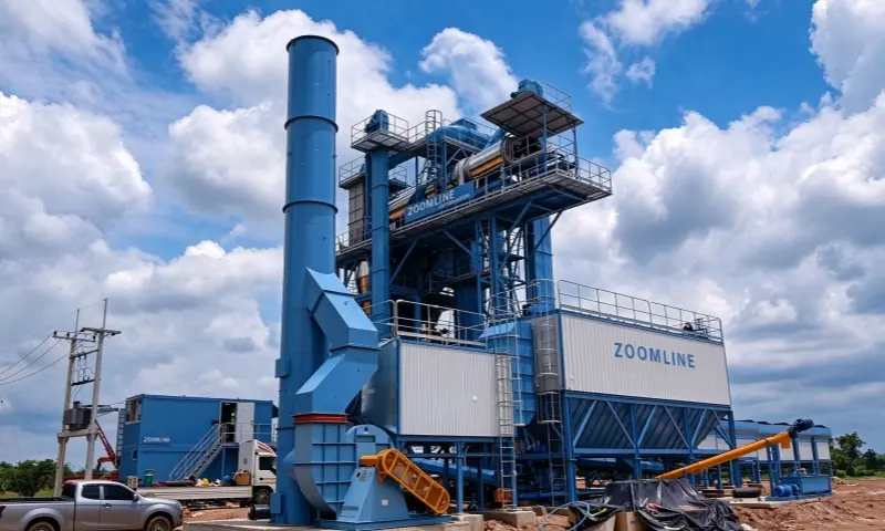
Compare Configuration Alternatives Using the Same Economic Model
Compare the initial investment, total life-cycle costs, cost per metric ton, and operational risks of different options. Maintain consistent output and quality requirements.
Select a configuration based on the project’s own economic analysis results; do not blindly trust claims that a particular type of equipment is universally more cost-effective. To ensure a fair comparison, input all candidate configurations into the same economic model (using identical annual output, quality requirements, evaluation period, and cost metrics). Discussing “which is cheaper” without reference to a specific project is often merely a marketing ploy. The final decision should be based on the specific question: “Given this project’s requirements and constraints, which configuration offers the best long-term economic performance and acceptable risk?”
It is important to note that upgrading or replacing existing equipment involves a different decision-making scenario than new construction investments; refer to “Should You Upgrade or Replace Your Existing Asphalt Plant?” for guidance.
Key Point: The configuration of an asphalt mixing plant must be determined based on project requirements and financial objectives.
A Practical Checklist for Evaluating an Asphalt Plant Investment
Translate the analytical methods outlined above into actionable investment review steps:
- Estimate actual annual production demand and the total project cycle: Based on contracts and sales forecasts, incorporate seasonal and utilization constraints to determine a realistic and achievable production range.
- Calculate the total initial capital investment and working capital requirements:Cover equipment, ancillary facilities, site preparation, installation and commissioning, transportation and customs clearance, pre-production preparations, and working capital, ensuring a consistent approach across multiple scenarios.
- Estimate operating costs using local data on fuel, labor, raw materials, and maintenance:Calculate costs separately under four categories—variable, fixed, maintenance-related downtime, and environmental compliance. First, standardize cost classifications and statistical boundaries to avoid double-counting, and use actual local data.
- Calculate the full life-cycle cost, cost per metric ton of mix, and break-even production volume:Standardize the evaluation period and cost metrics, and convert capital investment into operational unit costs and break-even production volume.
- Conduct stress tests under pessimistic scenarios to compare suitable asphaltbatching plant configuration options:Test sensitive variables such as demand, fuel prices, project duration, and cash collection to verify resilience under adverse conditions, and use a standardized model to compare different configurations.
- Before making the final investment decision, work with equipment suppliers and the finance team to review all assumptions in the model: confirm that key assumptions (future demand, oil prices, specifications, and environmental regulations) have been verified and that data definitions are consistent, then formulate the investment conclusion.
The purpose of this section is to provide a repeatable review process that eliminates the need for repetitive and complex formula derivations; with each completed step, the investment judgment converges based on the previous round of calculations, ultimately elevating “equipment procurement” to a “data-driven investment decision.”
Conclusion: Evaluate the Investment, Not Just the Equipment Price
The long-term economic viability of an asphalt plant equipment depends on accurate demand forecasts, comprehensive investment costs, actual capacity utilization rates, and full-cycle cash flow. Equipment quotes are merely the starting point of a lengthy economic analysis; what truly determines success or failure is the equipment’s ability to generate cash flow for the project under real-world demand and utilization conditions.
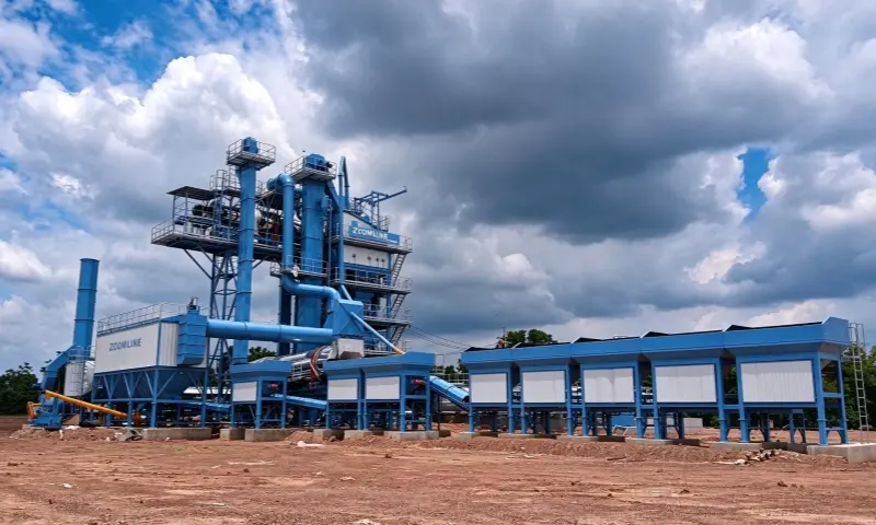
TCO (Total Cost of Ownership), cost-per-metric-ton calculations, break-even analysis, and multi-scenario stress tests collectively form a comprehensive feasibility assessment toolkit. They answer the same question from different angles—whether the investment is viable and whether the risks are acceptable—and corroborate one another; none can be overlooked.
The optimal investment solution is not the asphalt plant with the lowest quote or the highest nameplate capacity, but rather an equipment configuration that is highly aligned with the project’s production volume requirements and financial objectives. Only by shifting the focus of evaluation from “parameter comparison” to “economic analysis” can you make investment decisions that stand the test of time.
Call to Action
Planning to invest in an asphalt mixing machine? Share your target production capacity, project location, expected annual output, raw material conditions, and project timeline with ZOOMLINE. Our team can help you evaluate suitable asphalt mixing plant configurations and tailor solutions to your project’s specific needs.
Frequently Asked Questions
Q1:What Is the Total Cost of Ownership (TCO)of an Asphalt Plant?
TCO, or Total Cost of Ownership, requires the use of a unified statistical framework within a fixed evaluation period. It includes all upfront capital expenditures as well as ongoing operational, maintenance, and other costs, fully reflecting all economic expenditures from equipment procurement through decommissioning. It is the core metric for determining which option is “more cost-effective overall” rather than simply “cheaper to buy,” and serves as the foundational tool for making fair comparisons between different investment options. Note that TCO is a cost metric and is not equivalent to return on investment.
Q2:How Do You Calculate the Cost per Ton of Asphalt Mix?
Divide the total costs included in the statistical scope by the metric tons of marketable finished mixture produced during the same period. Most importantly, when comparing different options, the scope of cost calculation must remain consistent; otherwise, the comparison is invalid. It is necessary to clarify whether the scope is “on-site costs” or “full cost of the mixture,” ensuring that the time periods for both the numerator and denominator align, and that the denominator uses actual marketable output rather than rated capacity.
Q3:How Much Asphalt Does an Asphalt Mix Plant Need to Produce to Break Even?
The break-even output is determined by the total fixed costs and the marginal contribution per metric ton (selling price minus variable costs). The calculation logic differs between the “self-production for internal use” and “external sales” business models. The higher the fixed costs, the higher the minimum output threshold required; the greater the marginal contribution, the lower the break-even output. Break-even output is a core indicator for measuring the safety margin of an investment.
Q4: How Long Does It Take for an Asphalt Plant to Pay for Itself?
The payback period depends on the initial investment amount, actual capacity utilization rate, operating costs, and cash flow; there is no universal, fixed payback period. Insufficient utilization will significantly extend the payback period. The payback period should be assessed comprehensively using metrics such as NPV and IRR, and calculated under specific scenarios (base case, optimistic, and pessimistic), rather than relying on a generic industry average.
Q5:Is a Higher-Capacity Asphalt Plant More Economical in the Long Run?
Not necessarily. High-capacity equipment is only economically viable if market demand can absorb the additional output and if the additional equipment investment and operating costs can be spread across the increased production volume; if demand is insufficient, high-capacity equipment will drive up unit costs due to idling. Capacity selection should be based on “demand-driven production” and consider room for future expansion, rather than blindly pursuing higher capacity.