







How to Calculate Asphalt Hauling Costs and Improve Paving Efficiency
Introduction
For the vast majority of pavement construction contractors, the calculation of asphalt mixture transportation costs is often based simply on the distance in miles from the asphalt mixing plant to the construction site—it is assumed that as long as the transport distance remains constant, transportation costs will not vary significantly. However, asphalt transportation is by no means simply a matter of “distance × unit price”; rather, it is a highly coupled, closed-loop logistics system that includes loading, driving, unloading, the return trip, and waiting in line. Actual costs and the stability of material supply are not determined by transport distance alone. Fluctuations in fuel prices, queues for loading at the plant, traffic congestion, waiting times for unloading at the site, and driver work hour management—any one of these factors can continuously erode project profits and disrupt the rhythm of continuous paving.
Many projects encounter these pain points: pavers idling while waiting for material, vehicles clustering at the site and idling, significant temperature fluctuations in hot-mix asphalt, and repeated delays in finishing work. The root causes of these issues are mostly due to crude methods of calculating transportation costs, unreasonable configuration of the transport fleet, and a lack of synchronization between the mixing, transportation, and paving processes. Focusing solely on superficial measures—such as “dispatching a few more trucks” or “shortening a single trip”—often addresses symptoms rather than the root cause and may even lead to excess transport capacity and higher costs.
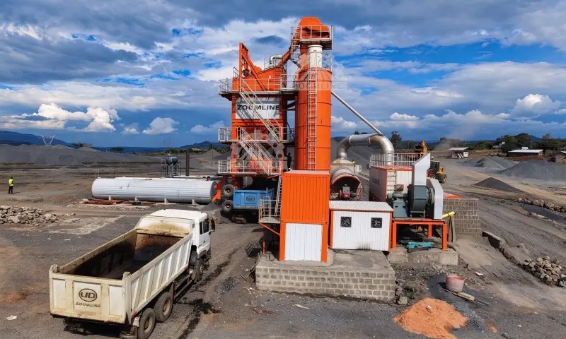
This article will provide a set of immediately implementable calculation methods: First, it explains the breakdown of asphalt transportation costs and establishes a unified accounting framework, providing a formula for calculating the transportation cost per metric ton of mix along with a complete calculation example; second, it offers the logic and formula for estimating the number of transport vehicles, helping projects configure a reasonable fleet based on supply requirements; third, it presents on-site scheduling optimization solutions to reduce transportation costs; finally, from the perspective of end-to-end bottlenecks, it analyzes under which operating conditions a mobile asphalt mixing plant can be evaluated as an alternative supply option, helping project managers ensure stable material supply, control transportation costs, and guarantee continuous paving.
Why Asphalt Hauling Distance Is More Than a Mileage Issue
Many people assume that “the farther the distance, the higher the cost.” While this logic is valid in principle, it simplifies a complex transportation issue into a single-factor judgment. In fact, even under the same mileage conditions, differences in road conditions, traffic light density, speed-limited sections, traffic controls, and loading/unloading wait times can result in significant variations in final transportation costs and vehicle turnaround efficiency.
Direct Transportation Costs Rise With Total Hauling Time
The direct variable costs of transportation primarily consist of three components: fuel consumption, vehicle maintenance and wear-and-tear costs, and driver labor costs based on hours worked. Among these, fuel consumption and driver labor costs accumulate linearly over time; every additional minute a vehicle travels or idles results in tangible expenses. Therefore, when calculating costs, it is essential to distinguish between three easily confused metrics: one-way distance (the single trip from the mixing plant to the construction site), round-trip mileage (a complete round trip), and actual travel time (the time actually spent on the road).
It is entirely possible for three routes to have the same mileage but vastly different travel times: one might be a smooth arterial highway where the average speed exceeds 60 kilometers per hour; another might be an urban route passing through the city, with numerous traffic lights, school zones, and traffic control points along the way, where the average speed may not even reach 30 kilometers per hour. For the same round-trip distance, the former might take one hour to complete, while the latter could take an hour and a half; naturally, fuel consumption per unit and driver labor hours would be completely different. If transportation costs are calculated based solely on mileage, cost estimates will deviate significantly from actual on-site conditions, leading to inaccuracies in subsequent fleet configuration and quotation calculations.
Longer Hauls Extend Truck Turnaround Time
To understand the impact of transport distance on a fleet, we must first establish the concept of “vehicle turnaround.” A complete material transport cycle consists of four stages: loading at the asphalt mixing plant (including waiting in line, weighing, and issuing a bill of lading); driving the loaded truck to the construction site; waiting on-site and unloading; and returning the empty truck to the asphalt mixing plant to wait in line for reloading. Together, these four stages constitute a single vehicle’s complete turnaround cycle. Longer transport distances and traffic congestion directly increase the duration of a single turnaround; slow loading and unloading also consume turnaround time.
This leads to a core principle that runs throughout this article: given a fixed material supply rate required for paving, the longer a single vehicle’s turnaround time, the more transport vehicles are needed to ensure a continuous and uniform supply of materials. In other words, the transport distance itself is not the problem; rather, the increased turnaround time caused by that distance is the issue—it directly determines how many trucks you need to maintain and how far apart you must space the dispatch intervals.
Unstable HMA Delivery Disrupts Continuous Paving
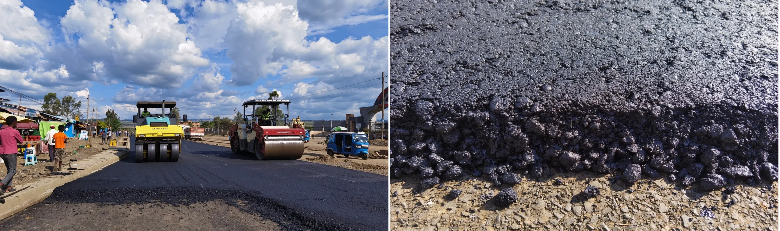
Beyond transportation costs, the stability of material supply also directly determines paving efficiency and pavement quality. When material supply is insufficient, the paver is forced to stop and wait for the mix, which can easily result in cold joints between the already laid layer and the newly paved section, directly affecting the quality of the pavement; conversely, if a large number of vehicles arrive at the paving site simultaneously, it causes traffic congestion and long periods of idling, which not only wastes fuel and labor hours but also causes the subsequent mix to remain in the truck bed and continue to cool.
Quality Risk Explanation: Excessive waiting times and temperature loss in the mix reduce the workability of hot-mix asphalt, increasing the risk of segregation and paving defects. It is important to emphasize that the severity of quality risks is related to multiple factors, including mix type, temperature control measures, transport duration, and on-site construction techniques. Waiting alone does not necessarily lead to quality issues, and quality fluctuations should not be attributed solely to the transportation process. Temperature control for hot-mix asphalt must strictly adhere to the temperature ranges specified in the project design, mix design, and construction specifications; there is no single, universal temperature standard that applies universally.
How to Calculate the True Cost of Asphalt Hauling
This section represents the core value of the entire article. The key to calculating asphalt transportation costs lies in establishing a unified set of accounting standards that incorporate all expenses related to the transportation cycle, ultimately yielding two critical figures: the cost per vehicle per trip, and the industry’s most crucial performance metric—the transportation cost per metric ton of asphalt mixture. Only by accurately calculating these two figures can subsequent fleet configuration, cost comparisons, and decision-making regarding implementation plans be based on reliable data.
Main Components of Asphalt Hauling Costs
Before calculating costs, it is essential to clarify which expenses should be included in transportation costs to avoid omissions or duplications. Typically, the components to be included are:
- Fuel, vehicle operation, and maintenance costs: Calculated based on actual mileage and idle time, these include expenses for fuel, tires, wear and tear, and scheduled maintenance.
- Driver labor costs: Billed by working hours; time spent driving, waiting in line, and waiting for unloading should all be included—not just the time “on the road.”
- Depreciation costs for company-owned vehicles or rental fees for leased vehicles: For company-owned vehicles, depreciation and insurance costs must be allocated; for leased vehicles, the contractual rental fee is included.
- Fixed time-based costs: Opportunity costs associated with time spent weighing, issuing invoices, and waiting in line at asphalt mixing plants for loading.
- Variable waiting costs: Additional costs resulting from waiting in line at paving sites or delays in unloading; the longer these waiting times, the lower the daily output per vehicle.
- Route-specific expenses: Expressway tolls, overweight permits, and special expenses incurred due to traffic restrictions or detours on specific road sections.
Calculate the Cost per Truck Trip
Establishing a standardized cost accounting ledger is essential for accurate cost calculations. The ledger should use a “single complete trip” as the smallest statistical unit, aggregating all expenses incurred during a single trip—including driver labor, fuel, tolls, and waiting time costs—and noting the corresponding tonnage and trip duration to facilitate subsequent allocation per metric ton.
It is particularly important to note: If the project employs an outsourced transportation fleet and a lump-sum turnkey contract model, care must be taken to avoid double-counting during cost calculations. Since the lump-sum unit price already includes transportation, loading/unloading, and waiting costs, items such as fuel, driver wages, and tolls should not be added again. Otherwise, the cost per metric ton will be artificially inflated, misleading subsequent decision-making.
Calculate Asphalt Hauling Cost per Ton
The transportation cost per metric ton is a core metric for comparing different operating conditions and alternatives. Two calculation formulas are provided; the accounting criteria must remain consistent:
Main Formula:
Transportation Cost per Metric Ton = Total Transportation Costs/Total Metric Tons of Mix Delivered
The main formula is suitable for overall accounting. It sums the costs of all transportation activities over a given period and divides them by the total metric tons of mix actually delivered to obtain the average cost per metric ton.
Simplified Formula (Suitable for Quick Estimates):
Transportation Cost per Metric Ton = Cost per Single Trip per Vehicle/ Effective Payload per Vehicle
The simplified formula is suitable for quick estimates during daily scheduling, provided that the cost per single trip per vehicle and the effective payload are calculated using the same accounting criteria; otherwise, the estimate will be inaccurate.
Important Principle: Whether using the main formula or the simplified formula, calculations must be based on the actual tonnage delivered as recorded on the weighbridge ticket, rather than the nominal load capacity listed on the vehicle’s nameplate. This is because the actual load capacity is reduced by factors such as weight limits, material spillage, and residual material in the hopper, while the nameplate load capacity represents only a theoretical upper limit. Only by using actual weighbridge data can the cost per metric ton be accurately and reliably calculated.
Calculate Hauling Cost
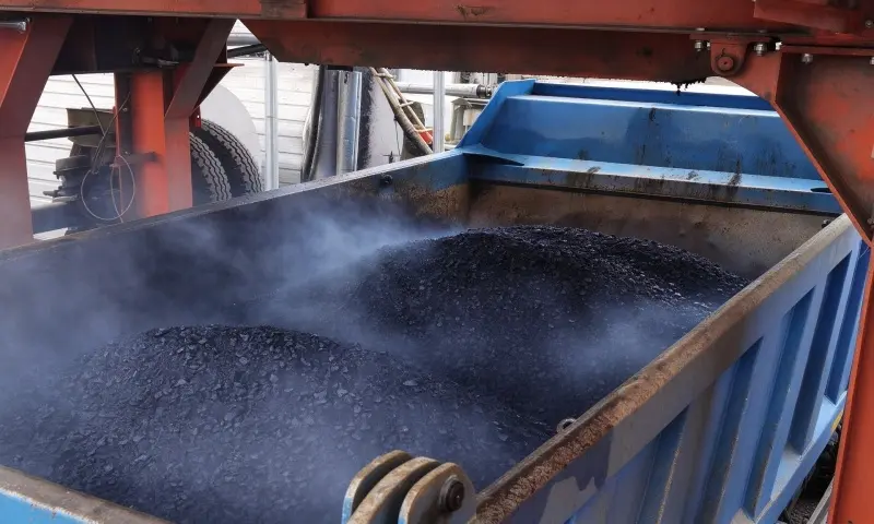
To help readers intuitively understand the calculation process, we provide a complete demonstration using a set of hypothetical data. The following figures are provided solely to illustrate the method; they do not represent any industry averages nor do they reflect ZOOMLINE’s actual operational data:
Assumptions:
- Effective payload per vehicle: 20 metric tons
- Cost per complete round trip per vehicle: $180
- Total number of trips: 10
- Total hot-mix delivered: 200 metric tons
Calculation Process: First, calculate the total transportation cost = cost per trip × total number of trips = 180 × 10 = $1,800; then calculate the cost per metric ton = total transportation cost ÷ total metric tons delivered = 1,800 ÷ 200. The final transportation cost per metric ton is $9/metric ton.
If verified using a simplified formula: Cost per trip per vehicle $180 ÷ Payload capacity per vehicle 20 metric tons = $9/metric ton. Both methods yield consistent results, indicating that the calculation logic is sound and the metrics are consistent.
Side-by-Side Scenario Comparison
The value of cost accounting lies in comparison. For the same project, the cost per metric ton will vary significantly under different transport distances, road conditions, and loading/unloading conditions. The table below summarizes comparisons of several typical operating conditions, with the focus on understanding how variables affect costs rather than memorizing specific figures:
| Comparison Scenario | Difference in Turnaround Time | Impact on Cost per Vehicle | Impact on Cost per Metric Ton |
| Short-Haul vs. Long-Haul Transport | Long-haul transport increases round-trip mileage and driving time | Rising fuel and labor costs per vehicle | Must be calculated in conjunction with payload; distance does not directly determine cost per metric ton |
| Smooth Traffic Conditions vs. Rush-Hour Congestion | Congestion significantly extends turnaround time | Increased fuel consumption due to idling and higher labor hours per vehicle | Decrease in daily trips per vehicle; cost per metric ton increases |
| Fast Loading vs. Queuing at the Terminal | Queuing increases wait time | Wait time costs are factored into per-vehicle turnaround time | Daily transport volume per vehicle decreases, and cost per metric ton increases |
| Fast Unloading vs. Waiting on-site | Waiting for unloading extends cycle time | On-site waiting time is factored into per-vehicle costs | Payload remains unchanged, but daily trips per vehicle decrease |
Comparison Conclusion: Mileage is only one of the factors affecting costs; total turnaround time is a more reliable benchmark for comparison. Whether the transport distance is long or short, as long as the turnaround time per vehicle is short and the number of trips completed per day is high, there is an opportunity to reduce the cost per metric ton. Therefore, before drawing any conclusions about costs, one must rely on clear data assumptions and a complete calculation process; one cannot simply conclude that “long-distance transport is necessarily more expensive” or that “reducing waiting time will consistently save a certain percentage of costs”—such conclusions must be verified with actual data.
How to Estimate Truck Requirements for Continuous Paving Operations
Estimating fleet size is one of the aspects of transportation management most prone to being decided on a whim. This section provides a scientific estimation method based on material supply requirements, per-truck load capacity, and turnaround time, enabling readers to calculate the theoretical minimum number of vehicles using a formula and to set aside a reasonable buffer for fluctuation risks.
Key Variables for Haul Fleet Planning
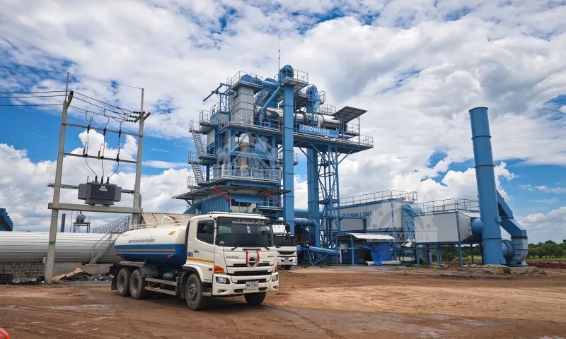
Before performing the calculations, you must first collect all of the following key parameters; none can be omitted:
- Hourly production capacity of the asphalt mixing plant (metric tons per hour): This determines the upper limit of material supply; if production capacity is insufficient, even the largest fleet will be ineffective.
- Hourly supply rate of mix required for paving operations (metric tons per hour): Determined by paving width, thickness, and paving speed, this is the target value for fleet planning.
- Actual payload per vehicle: Based on the actual weight recorded on the scale, not the rated load capacity.
- Full vehicle turnaround time (in minutes): The entire cycle from loading to returning to the queue.
- Effective shift duration and number of available vehicles: How many hours of actual construction are possible per day and how many vehicles are available.
- On-site mix buffer stock (if applicable): If the site allows for a small amount of stockpiled material, this can help buffer fluctuations in material supply to some extent.
Measure & Calculate Total Truck Cycle Time
Turnaround time is the most critical—and also the most difficult to measure accurately—variable in the formula. A complete turnaround includes all stages; it is essential to track it consistently according to the criteria below (a complete definition is provided in this section and will not be repeated in subsequent chapters):
- Queuing at the asphalt mixing plant, loading, weighing, and document registration
- Loaded vehicles traveling to the construction site
- Waiting on-site, positioning, and unloading
- Empty vehicles returning to the asphalt mixing plant and re-entering the queue
Practical Recommendation: Turnaround time must be measured based on actual data recorded on-site during each shift; dispatchers or drivers can be assigned to log times at each stage. Do not directly use the theoretical travel time from map navigation apps—this does not account for waiting times during queuing and unloading, nor does it reflect peak-hour traffic congestion or road closures. Only by relying on actual measured data can the fleet size be accurately calculated.
Formula for Minimum Number of Circulating Trucks
Once the feed rate, load capacity, and turnaround time are known, the following formula can be used to estimate the theoretical minimum number of vehicles required to maintain the supply:
N = Floor [ (R × T) ÷ (Q × 60) ]
Parameter Explanations:
- R: Required mix supply rate per hour (metric tons/hour)
- T: Total turnaround time per vehicle (minutes)
- Q: Effective payload per vehicle (metric tons per trip)
The logic behind the formula is as follows: The hourly supply requirement R must be met by a series of vehicles working in relay; if each vehicle can carry Q metric tons per trip and completes one trip every T minutes, then the number of metric tons a single vehicle can deliver in one hour is Q × 60 ÷ T. Dividing the hourly demand R by the hourly transport capacity per vehicle yields the required number of vehicles, which is then rounded up.
Important Note: The calculated result represents the minimum number of vehicles required to maintain a steady supply under stable operating conditions, assuming consistent turnaround times, compliance with load requirements, and uninterrupted vehicle operation. This figure does not include backup vehicles for emergency repairs. In actual projects, if road conditions fluctuate significantly, vehicle failure rates are high, or construction is subject to unexpected interruptions, the need for standby vehicles must be assessed separately in light of project volatility risks. It is not sufficient to simply assume a “fixed increase of 1–2 vehicles”—the number of standby vehicles should be determined based on historical data and an actual assessment of on-site risks.
Calculate Required Fleet Size
Here is a specific example demonstrating how to use the formula:
- Required paving feed rate: 120 metric tons per hour
- Effective payload per vehicle: 20 metric tons
- Total turnaround time: 60 minutes
Substituting into the formula:
N = Floor [ (120 × 60) ÷ (20 × 60) ] = Floor [7,200 ÷ 1,200] = Floor 6 = 6 vehicles.
In other words, theoretically, a minimum of 6 shuttle trucks is required to maintain a feed rate of 120 metric tons per hour.
Additional Note: This figure of 6 trucks is derived under ideal conditions—a 60-minute turnaround time, a full load of 20 metric tons, and uninterrupted operation. If the actual turnaround time is extended to 70 minutes due to traffic congestion or queuing, the number of vehicles will need to be increased; if the site allows for a certain amount of buffer stock, or if the paving speed can be temporarily reduced, then the required number of vehicles can be slightly adjusted. Additionally, if road conditions are unstable or vehicle failure rates are high, the addition of standby vehicles may be evaluated separately; however, standby vehicles are not part of the circulating feed fleet, and the two must be accounted for separately.
Risks of Under-Sizing or Over-Sizing the Fleet
A larger fleet is not necessarily better, nor is a smaller one necessarily more cost-effective; both extremes come at a cost:
Insufficient number of transport trucks: Mix supply becomes intermittent, paving machines frequently stop to wait for material, cold joints are likely to form, paving capacity drops significantly, and pavement quality is compromised. In such cases, the savings on vehicle costs are often far outweighed by the losses resulting from downtime and quality-related rework.
Excessive number of transport trucks: Vehicles crowd the paving site, forming long queues and idling for extended periods, resulting in wasted driver labor hours and fuel consumption, which directly drives up transportation costs. At the same time, the mixture remaining in the truck bodies continues to cool, increasing the risk of segregation—ultimately compromising pavement quality.
Optimal Scenario: Mixers arrive at even intervals, with dispatch rhythms matched to the paver’s laying speed—ensuring neither material shortages nor traffic congestion. This “equilibrium point” is achieved through precise calculation of turnaround times and dynamic scheduling.
How to Reduce Asphalt Hauling Costs Without Disrupting Paving
After calculating costs and optimizing the fleet, true cost reduction and efficiency gains depend on meticulous on-site scheduling. This section focuses on practical scheduling methods; it does not repeat the definition of turnaround time, and all content is geared toward operations that can be immediately implemented on-site. Cost reduction is not simply about driving down prices or cutting back on vehicles, but rather about optimizing waiting times and idle periods at every stage to maximize output from the same resources.
Optimize Routes Based on Actual Travel Time, Not Just Mileage
When planning transport routes, focus on actual travel time rather than straight-line mileage. Simultaneously consider factors such as road closures, weight restrictions, construction-related traffic controls, and speed reductions during morning and evening rush hours—a route that appears to be the shortest may actually be less time- and cost-efficient than a slightly longer but unobstructed route if it is frequently congested or subject to traffic restrictions. At the same time, allow for a reasonable time buffer to account for predictable delays (such as rush hour traffic or construction-related traffic controls) to prevent unexpected situations from disrupting the dispatch schedule.
Cut Plant Queuing and Waiting Time
Queues at mixing plants are a significant hidden source of transportation costs. To reduce this waiting time, confirm the mix type, total volume, and dispatch schedule in advance with the asphalt mixing plant dispatcher and on-site foreman to ensure loading preparations are in place ahead of time. Simultaneously, optimize the workflow between weighing, document issuance, and loading to minimize document processing time. Also, be careful not to dispatch more vehicles at once than the plant’s loading capacity can handle; otherwise, vehicles will be left idling at the plant, wasting transport capacity.
Coordinate Dynamic Truck Dispatch With Live Paving Progress
Scheduling departures at fixed intervals may seem convenient, but it can actually lead to uneven material supply. A more scientific approach is dynamic, on-demand scheduling: maintain a log recording each vehicle’s departure, arrival, completion of unloading, and return to the asphalt mixing plant to track each vehicle’s progress in real time; When paving speed slows down, traffic congestion occurs, or vehicles are backed up on-site, promptly extend the dispatch intervals; when paving speeds up or the paver is about to run out of material, appropriately increase the frequency of dispatches. Through this dynamic adjustment, ensure that the material delivery rhythm consistently aligns with the actual paving progress.
Optimize On-Site Unloading Routes and Traffic Organization
The organization of loading and unloading at the paving site directly affects the unloading wait time for each vehicle. Fixed routes for vehicle entry, maneuvering into position, unloading, and exit should be planned in advance to prevent vehicles from crisscrossing the site haphazardly; establish a unified communication mechanism among dispatchers, drivers, paver operators, and site supervisors to ensure information is synchronized across all stages; set up a dedicated waiting area near the unloading point so that vehicles awaiting unloading can park in an orderly manner, preventing blockages at the unloading point and delays along the entire unloading line.
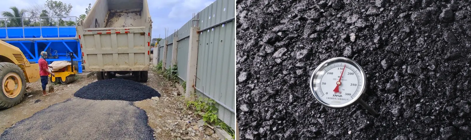
Track KPIs and Continuously Optimize Logistics After Every Shift
Cost reduction and efficiency improvement are an ongoing, iterative process that relies on data support. The following core KPIs should be tracked for each shift:
- Planned turnaround time vs. actual turnaround time
- Transportation cost per vehicle/per metric ton
- Metric tons delivered per hour
- Paver wait time for material
- Number of trips completed per shift
Optimization Logic: Prioritize using data to identify bottlenecks—whether it’s slow loading, traffic congestion, or unloading delays—and then make targeted adjustments, rather than simply increasing the number of leased or purchased transport vehicles. Data tells us “where the problem lies” in the process, rather than making every link in the chain take the blame.
Align Asphalt Plant Output, Hauling Capacity and Paving Rate
The previous sections addressed cost estimation, fleet configuration, and on-site scheduling, respectively. This section examines these elements within the context of the entire construction chain. The upper limit of the entire asphalt pavement construction chain is determined by three rates: the asphalt mixing plant’s production capacity, effective transportation capacity, and paving consumption rate. These three factors must be coordinated and aligned; the slowest link in the entire chain represents the project’s production bottleneck and is the key factor ultimately determining the project’s progress.
Identify the True Bottleneck Before Adding More Resources
When problems arise with material supply or paving, don’t reflexively “buy a few more trucks.” First, determine exactly where the bottleneck lies:
- Insufficient transport capacity: This manifests as the asphalt mixing plant being forced to reduce its output; otherwise, a large number of trucks would be backed up in line at the plant. In this case, the bottleneck is in transportation, and only increasing effective transport capacity makes sense.
- Loading bottleneck: There are enough trucks, but the asphalt mixing plant’s loading speed is slow, causing vehicles to queue for extended periods on-site. In this case, the problem lies in the loading process; adding more trucks will only worsen congestion at the plant.
- Paving bottleneck: The paver cannot consume the mix fast enough to keep up with the supply rate, causing material to pile up at the paving site. In this case, the problem lies in the paving process; increasing the supply will only lead to traffic congestion at the site.
Key Conclusion: Simply increasing the number of transport trucks cannot resolve bottlenecks such as slow loading at the asphalt mixing plant or insufficient paver capacity. Before allocating additional resources, it is essential to pinpoint exactly where the bottleneck lies; otherwise, the greater the investment, the greater the waste.
Reassess Your Asphalt Supply Source When Long-Distance Hauling Becomes Unsustainable
If a project is chronically constrained by long-distance transportation, it is worth pausing to reassess the overall material supply plan. Typical warning signs that trigger such an assessment include: the construction site being too far from a fixed asphalt mixing plant; complex scheduling due to multiple dispersed work sites; recurring delays in material turnover; and continuous disruption to paving continuity. When these signs recur, it indicates that the fundamental assumption of “transporting materials from a distant mixing plant” may no longer be economically viable.
When Is a Mobile Asphalt Plant a Worthwhile Project Option?
When long-distance transportation becomes a persistent pain point, the idea of “local production” often comes to mind. Mobile asphalt mixing plants are precisely the solution designed for such scenarios. Suitable operating conditions for evaluation include: linear road construction projects (where the paving front continuously advances and the supply point must follow), projects with remote access roads and poor conditions, projects with dispersed work sites, and projects where long-distance transportation results in unstable material supply.
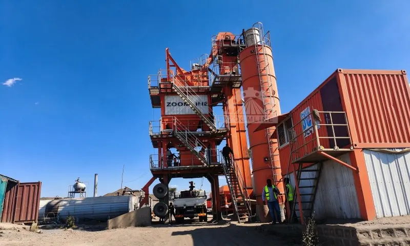
However, the evaluation cannot focus solely on the single benefit of “local material supply.” A comprehensive assessment is essential: total project duration, estimated total output, frequency of asphalt mixing plant relocations, installation and permitting procedures, and freight costs for transporting raw materials to the on-site mixing point. Then, compare the total costs of the two approaches—the total cost of on-site production using a mobile plant versus the total cost of long-distance transportation from a stationary asphalt mixing plant. Only by factoring in one-time investments, operating costs, relocation costs, and material transshipment costs can a reliable decision be made.
Objective Note: Mobile asphalt mixing plants cannot eliminate all transportation risks; they merely shorten the distance between the mixing point and the paving site by replacing long-distance transport with on-site production. However, raw materials may still need to be transported long distances to the site. Therefore, they do not automatically save money on every project. Decisions must be made only after comparing the complete comprehensive costs, and one should avoid viewing “mobile plants” as a universal solution.
Practical Asphalt Hauling Cost & Paving Efficiency Checklist
To help project managers conduct quick self-checks, the key points from the full text have been compiled into a ready-to-use checklist. By reviewing each item, you can quickly identify weaknesses in transportation management:
□ Have you calculated the actual per-truck transportation cost and the transportation cost per metric ton of mix?
□ Is route planning based on actual travel times and real-world traffic conditions?
□ Are vehicle load data derived from weighbridge tickets rather than the rated load capacity on the nameplate?
□ Do cycle time statistics include all stages—loading, queuing, unloading, and return trips?
□ Can the number of vehicles in the transport fleet consistently meet supply demands, and are backup vehicles evaluated separately?
□ Can the asphalt mixing plant consistently achieve its designed hourly production capacity?
□ Is the arrival schedule of transport trucks aligned with real-time paving progress?
□ Are transportation costs, turnaround times, and waiting delays reviewed after each shift?
Core Approach: Collect real-time on-site data → Scientifically calculate costs → Streamline coordination between mixing, transportation, and paving → Continuously refine logistics scheduling plans. Only by optimizing this workflow can transportation costs be controlled and paving efficiency guaranteed.
Conclusion: Calculate, Coordinate, and Optimize Asphalt Hauling
Accurately calculating transportation costs is the foundation for safeguarding the profitability of pavement projects; rationally planning fleet size and managing turnaround times are key to ensuring continuous paving. The core of this article is to view asphalt mixing, logistics, and on-site paving as an integrated system—any disruption in one link will affect overall efficiency. Conversely, as long as costs are accurately calculated, the fleet is adequately staffed, scheduling is optimized, and the “three speeds” are aligned, transportation will no longer be a hidden cost black hole for the project but will instead serve as a stabilizer that ensures project progress. After estimating delivery and paving costs, you need to decide whether purchasing or self-production is better. See our make-or-buy decision for asphalt supply for a complete evaluation framework.
If long transport distances, unstable material supply, and frequent changes in work locations continue to hinder your paving operations, please contact ZOOMLINE. We will tailor a material supply solution—whether using a stationary or mobile asphalt mixing plant—based on your project requirements, expected production capacity, and on-site conditions. ZOOMLINE offers a complete range of asphalt production equipment solutions, from stationary to mobile, to help you stabilize your entire paving process starting from the material supply source.
Frequently Asked Questions (FAQ)
Frequently asked questions regarding transportation costs and paving efficiency are summarized below:
How Do You Calculate Asphalt Hauling Cost per Ton?
Divide the total freight cost by the total tonnage delivered. A simplified method is to divide the cost per truck per trip by the truck’s payload capacity. During the calculation process, ensure consistency in statistical criteria; prioritize actual tonnage as determined by weighing rather than the rated load capacity.
How Does Hauling Distance Affect Asphalt Paving Efficiency?
It primarily affects paving by extending vehicle turnaround time, reducing the stability of material supply, and introducing risks related to mix temperature control. Transportation distance itself does not directly determine cost levels; road conditions, waiting times in traffic, and loading/unloading speeds have equally significant—if not greater—impacts.
How Many Trucks Are Needed for an Asphalt Paving Project?
Substitute the turnaround time, hourly feed rate, and load capacity per truck into the formula N = round up [(R × T) ÷ (Q × 60)] to calculate the minimum number of vehicles required for a cycle. This figure is based on the assumption of stable operating conditions; when determining actual configurations, standby vehicles must be assessed separately in light of fluctuations in road conditions.
What Is Asphalt Truck Cycle Time?
It refers to the duration of a complete cycle, starting from when the vehicle enters the asphalt mixing plant to queue for loading, through loading, driving with a full load, unloading at the site, and returning to the asphalt mixing plant after unloading to wait for the next load. It encompasses all stages: loading, driving, unloading, the return trip, and queuing.
How Can You Reduce Asphalt Truck Waiting Time?
Finalize dispatch schedules in advance, optimize the loading sequence at the asphalt mixing plant, standardize on-site traffic flow, continuously track turnaround KPIs, and dynamically adjust dispatch rhythms based on actual data to ensure the material delivery pace aligns with paving progress.
When Should a Contractor Consider a Mobile Asphalt Plant?
It should be evaluated for projects with remote construction sites, scattered locations, persistently high long-distance transportation costs, or unstable material supply. Before making a decision, compare all comprehensive costs—including project duration, total output, relocation costs, and raw material transshipment—to confirm that the mobile plant solution is indeed more economical.